My First Blog - Practice with Spatial Data

Code

library(tidyverse)

── Attaching packages ─────────────────────────────────────── tidyverse 1.3.2 ──
✔ ggplot2 3.3.6      ✔ purrr   1.0.1 
✔ tibble  3.1.7      ✔ dplyr   1.0.10
✔ tidyr   1.2.0      ✔ stringr 1.4.0 
✔ readr   2.1.2      ✔ forcats 0.5.1 
── Conflicts ────────────────────────────────────────── tidyverse_conflicts() ──
✖ dplyr::filter() masks stats::filter()
✖ dplyr::lag()    masks stats::lag()

Code

library(readxl)
library(rnaturalearth)
library(rnaturalearthdata)


Attaching package: 'rnaturalearthdata'

The following object is masked from 'package:rnaturalearth':

    countries110

Code

library(dplyr)

Malaria <- read.csv("National_Unit_data.csv")

Incidence<- Malaria%>%
  filter(Metric == "Infection Prevalence" & Year == "2019")%>%
  mutate(Prevalence = Value)%>%
  select(c(ISO3, Prevalence))

Code

world_map <- ne_countries(scale = 'medium', returnclass = "sf")

map_data <- world_map %>%
  left_join(Incidence, by = c("iso_a3" = "ISO3"))

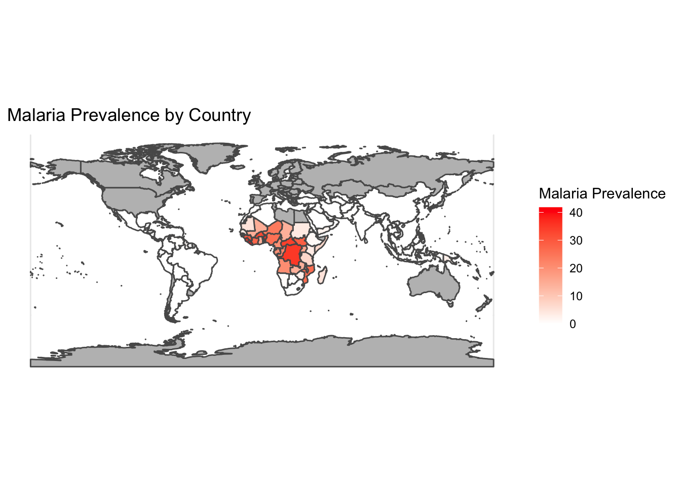
Code

ggplot() +
  geom_sf(data = map_data, aes(fill = Prevalence)) +
  scale_fill_gradient(low = "white", high = "red", na.value = "gray", name = "Malaria Prevalence") +
  theme_minimal() +
  theme(axis.text = element_blank(), axis.ticks = element_blank(), axis.title = element_blank()) +
  labs(title = "Malaria Prevalence by Country")

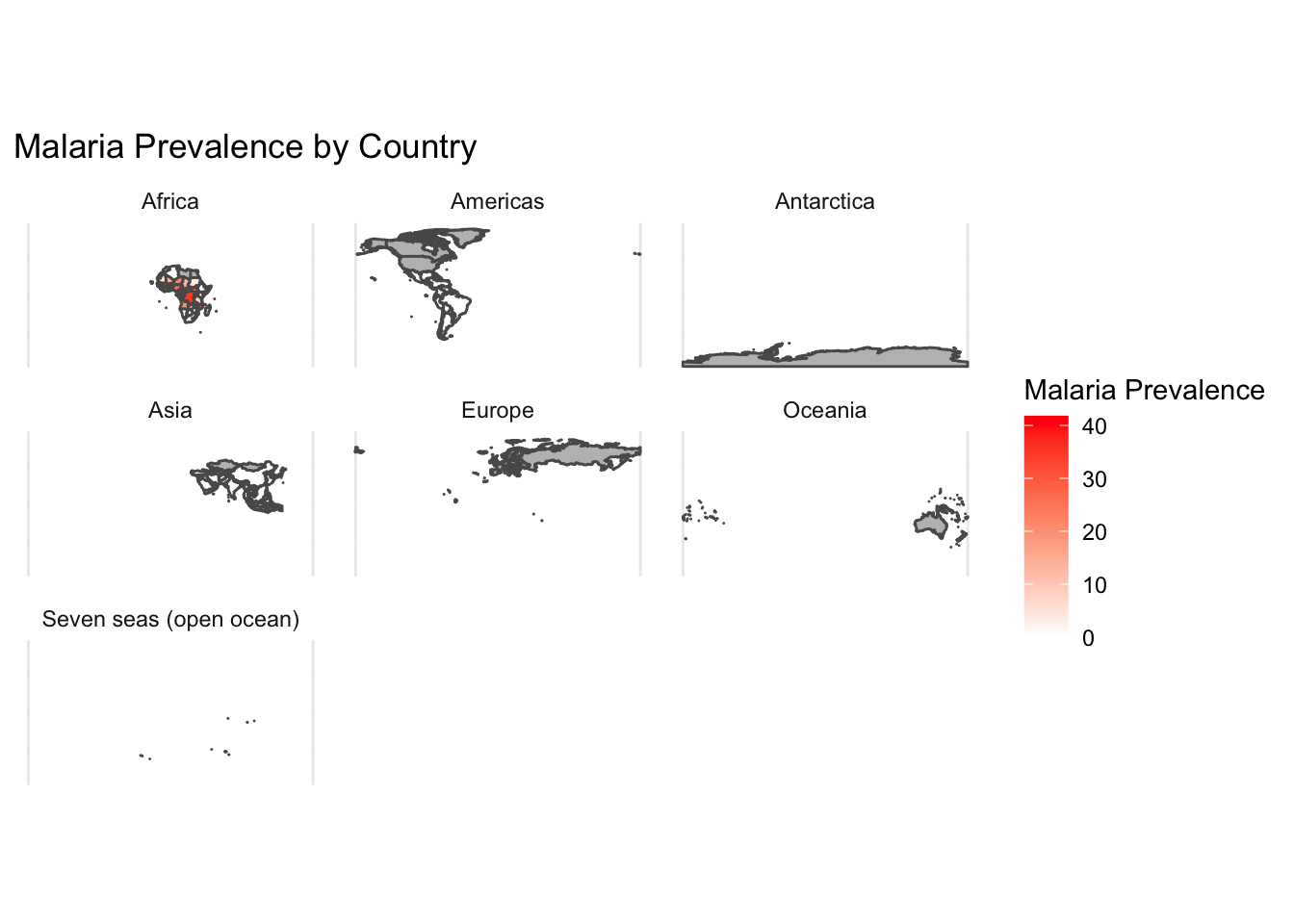
Code

ggplot() +
  geom_sf(data = map_data, aes(fill = Prevalence)) +
  scale_fill_gradient(low = "white", high = "red", na.value = "gray", name = "Malaria Prevalence") +
  theme_minimal() +
  theme(axis.text = element_blank(), axis.ticks = element_blank(), axis.title = element_blank()) +
  labs(title = "Malaria Prevalence by Country") +
  facet_wrap(~ region_un)

Code

# # Filter to only include infection prevalence data for a specific year
# Year <- 2019
# Incidence <- Malaria %>%
#   filter(Metric == "Incidence Rate" & Units == "Cases per Thousand" & Year == Year) %>%
#   mutate(Incidence_Rate = Value) %>%
#   select(c(ISO3, Incidence_Rate))
# 
# # Get world map data with medium scale
# world_map <- ne_countries(scale = "medium", returnclass = "sf")
# 
# # Join incidence data with world map data
# map_data <- world_map %>%
#   left_join(Incidence, by = c("iso_a3" = "ISO3"))
# 
# # Create the choropleth map using ggplot2
# ggplot() +
#   geom_sf(data = map_data, aes(fill = Incidence_Rate)) +
#   scale_fill_gradient(low = "white", high = "red", na.value = "gray", name = "Malaria Incidence Rate") +
#   theme_minimal() +
#   theme(axis.text = element_blank(), axis.ticks = element_blank(), axis.title = element_blank()) +
#   labs(title = paste0("Malaria Incidence Rate by Country in ", Year))

Code

library(tidyverse)
library(readxl)
library(rnaturalearth)
library(rnaturalearthdata)
library(dplyr)
library(gganimate)
library(transformr)

Malaria <- read.csv("National_Unit_data.csv")

Incidence <- Malaria %>%
  filter(Metric == "Infection Prevalence" & Year >= 2010 & Year <= 2020) %>%
  mutate(Year = as.factor(Year),
         Prevalence = Value)

world_map <- ne_countries(scale = "medium", returnclass = "sf")

map_data <- world_map %>%
  left_join(Incidence, by = c("iso_a3" = "ISO3"))

p <- ggplot() +
  geom_sf(data = map_data, aes(fill = Prevalence)) +
  scale_fill_gradient(low = "white", high = "red", na.value = "gray", name = "Malaria Prevalence") +
  theme_minimal() +
  theme(axis.text = element_blank(), axis.ticks = element_blank(), axis.title = element_blank()) +
  labs(title = "Malaria Prevalence by Country") +
  transition_states(Year, transition_length = 2, state_length = 2)

animate(p, fps = 25, width = 800, height = 500)

Warning in lapply(row_vars$states, as.integer): NAs introduced by coercion

Warning in f(..., self = self): NAs introduced by coercion